Welcome to Statistics

I greet you this day,
First: read the notes.
Second: view the videos.
Third: solve the questions/solved examples.
Fourth: check your solutions with my thoroughly-explained solutions.
Fifth: check your answers with the calculators as applicable.
Comments, ideas, areas of improvement, questions, and constructive criticisms are welcome. You may contact me.
If you are my student, please do not contact me here. Contact me via the school's system.
Thank you for visiting.

Samuel Dominic Chukwuemeka (Samdom For Peace) B.Eng., A.A.T, M.Ed., M.S

Introductory Statistics

---

Objectives

Students will:
(1.) Discuss statistics.
(2.) Discuss the basic terms used in statistics.
(3.) Discuss the reasons for studying statistics.
(4.) Define data.
(5.) Identify the population, sample, and individual in scenarios.
(6.) Identify the statistic and/or parameter in scenarios.
(7.) Discuss the statistical process.
(8.) Classify variables as qualitative or quantitative.
(9.) Classify quantitative variables as discrete or continuous.
(10.) Classify variables based on the level of measurement of the variable.

Definition

Statistics is the science that deals with the:
Collection
Organization
Presentation
Analysis and
Interpretation of data so as to make the right decision and the right conclusion.

The main reason for studying statistics is to make the right decision and the right conclusion.
The goal of learning statistics is to distinguish between statistical conclusions that are likely to be valid and those that are seriously flawed.

Teacher: Would you not like to make the right decision in anything you want to do?
What are some of those things? 😊😊😊 Note students responses.
Would you want to be able to differentiate between results that are valid and results that are flawed?
Would you want to be able to prevent any sources of bias when making important decisions?
Welcome to Statistics!

There are basically, two types of statistics:
Descriptive Statistics and
Inferential Statistics

Descriptive Statistics is the science that deals with the collection, organization, and presentation of data.
Inferential Statistics is the science that uses methods that takes the results obtained from a sample, infers it on the population, and measures the reliability of the results.

Why do we learn Statistics?

(1.) The media uses statistics to predict election polls such as the Presidential election and nominate people for awards among others.

Example 1: President Barack Obama vs Governor Mitt Romney 2012 Presidential Poll - Gallup Polls

Example 2: Who do Americans blame for the Saturday, December 22, 2018 partial government shutdown?
More Americans blame President Trump for government shutdown - Reuters/Ipsos Polls

Discuss some statistics in those links.
For Example 2, read the second to the last paragraph.
Discuss more real-world examples if time is available.
Ask students to research more "valid" sites.
Hmmmm...how do you know if a website is valid? How do you know if a website is not biased?

(2.) School administrators use statistics to know the performance of the schools in their district, and make decisions as necessary.

Example 3: The Nation's Report Card - The National Assessment of Educational Progress (NAEP)

Discuss how NAEP obtain their data (data collection) to rate schools in each state.
Discuss some statistics based on their results.

(3.) Health professionals use statistics to know how different people react to different medicines.

(4.) Teachers use statistics to know how to meet the learning needs of their students.

(5.) People use statistics to make informed or decisions on who to marry (typical in Africa and India), what professor's class to take (typical in the United States where "unknown people" insult their teachers and professors), what car to buy, and what school to attend among others.

Data

Data is the list of observed values for a variable.
Data is the fact used to make a conclusion or decision.
It is also referred to as Information.
It is collected from a survey, an experiment, and a historical record among others.
It can be numeric (numbers) such as age, weight, etc. It is more than just numbers, because it has context.
It can also be non-numeric such as color, gender, etc.
The process of posing a question, collecting data, analyzing data, and interpreting the data is known as a Data Cycle.
Data vary. It changes within an individual. It also changes among individuals.
Understanding the variablity of data is very important in statistics.
Statistical studies rely on two major concepts: Data and Variation.
Collecting data about something involves a study of that thing.
This study could be measured or observed.
That leads us to...

Population, Sample, and Individual

Population is the entire group of individuals or thing that is being studied.
It contains all subjects of interest.
Example: All student matadors (Arizona Western College students).

Sample is a proper subset (part) of the population being studied.
It contains some members of the population.
It contains some of the subjects of interest.
Example: AWC students in South Yuma campus.

Bring it to Algebra: what is the difference between a subset and a proper subset?

Individual is a member of the population being studied.
It is a subject of interest.
Example: An AWC student in San Luis campus.

Exercise 1
For each of these scenarios, identify the population, sample, and individual.

(1.) A 2012 survey of 100 million Nigerians in Nigeria found that they would prefer the South to secede from the North.

Show/Hide Answer

(2.) 300 ladies aged 19 to 35 who live in the United States were contacted in a poll.
The poll asked whether they use abstinence as a form of birth control.
Hmmmm...what do you think the results would be?

Show/Hide Answer

(3.) Naboth randomly sampled 125 plants in his farm on June 30 and weighed the chlorophyll in each plant.

Show/Hide Answer

From Question 1 in Exercise 1

Assuming 95 million Nigerians out of 100 million Nigerians said they were ready to secede immediately.
This means that 95\% of the 100 million Nigerians that were surveyed are ready for the secession immediately.
This describes the results of the sample without making any conclusions about the population. (Descriptive Statistics).
Note the population here is the entire Nigerian population.
This leads us to...

Statistic and Parameter

Statistic is a numerical summary of a sample.
A statistic is often referred to as an estimator.

Please note: It is "Statistic", not "Statistics".
No, Statistic is not the singular form of Statistics! 😊😊😊

In our example, the 95% is the statistic.
Suppose we now take this 95% and extend it to the entire Nigerian population. (Inferential Statistics).
Assume we now say that 95% of all Nigerians in Nigeria said they were ready to secede immediately, then the
95% becomes the parameter.

Parameter is a numerical summary of a population.

Did you notice how we went from Descriptive Statistics to Inferential Statistics?
Did you notice how we went from Sample to Population?
Did you notice how we went from Statistic to Parameter?
Is it making sense?

Because a statistic is usually known while a parameter is usually unknown, a statistic is a measurable estimator of an often unknown population parameter.
A statistic is represented by English letters while a parameter is represented by Greek letters.
For example:
(a.) Sample mean (statistic) is represented by $\bar{x}$
Population mean (parameter) is represented by μ

(b.) Sample standard deviation (statistic) is represented by s
Population standard deviation (parameter) is represented by σ

(b.) Sample variance (statistic) is represented by s²
Population variance (parameter) is represented by σ²

In rare cases, the parameters may be represented by English letters.
(d.) Sample proportion (statistic) is represented by $\hat{p}$
Population proportion (parameter) is represented by p

Exercise 2
For each of these scenarios, identify whether the underlined is a statistic or parameter.

(4.) A sample of London residents were surveyed and it was found that 85% had a bachelors degree or higher.

Show/Hide Answer

(5.) In a study of all 16000 students of Divine Mercy Academy, it was found that 99% of them speak in tongues.

Show/Hide Answer

(6.) By 2014, around 38% of all mobile phone users were smartphone users.
By 2018, this number is expected to reach over 50%.
(Number of mobile phone users worldwide from 2015 to 2020 (in billions) - Statista - The Statistics Portal)

Show/Hide Answer

(7.) 26 of the 50 states in the United States voted for Barack Obama in the 2012 Presidential Elections.
(Presidential Election Results - NBC News)

Show/Hide Answer

(8.) A homeowner in the City of Truth or Consequences, New Mexico measured the voltage supplied to his home on 6 days of a given week, and found that the average value was 120 volts.

Show/Hide Answer

(9.) The Federal Republic of Nigeria has 36 states.
Assume the areas of 3 of the Southeastern states are added and the sum is divided by 3, the result is 5301.70566 square kilometers.

Show/Hide Answer

(10.) Median weekly earnings of full-time workers were $887 in the third quarter of 2018.
Women had median weekly earnings of 796, or 81.8 percent of the 973 median for men.
(Usual Weekly Earnings of Wage and Salary Workers Third Quarter 2018 - Bureau of Labor Statistics)

Show/Hide Answer

(11.) Of the 100 United States Senators, 77 of them voted for the Iraq war.
(Senate Roll Call: Iraq Resolution - The Washington Post)

Show/Hide Answer

(12.) A study from Harvard University researchers found that of 93,600 women aged between 25 and 42, three or more servings of berries per week may slash the risk of a heart attack by 33%. (Berries may lower women’s heart attack risk - Harvard School of Public Health published in the January 14, 2013 issue of the American Heart Association’s (AHA) journal Circulation)

Show/Hide Answer

Statistical Process

Statistics is a science because its process follows the scientific method.
The basic steps of a statistical process is:

(1.) Identify the research objective
What do you want to find out about?
What are the necessary questions to be asked?
What is the population of the study?

(2.) Collect the data needed to answer the questions
Use appropriate data collection techniques. (Data Collection)
Gaining access to an entire population is usually difficult.
So, a sample is needed.
How random did take your sample? (Sampling Methods)
How large is your sample size?

(3.) Describe the data
Obtain a descriptive statistics of your sample data. (Descriptive Statistics)
Organize your data. (Data Organization)
Present your data properly. (Data Presentation)
Analyze your data. (Data Analysis)

(4.) Perform Inference
Apply appropriate techniques to extend the results of your sample data to the population of your study. (Inferential Statistics)
If the sample fairly represents the population as a​ whole, then it is reasonable to make inferences from the sample to the population.
Report a level of reliability of the results.
What is the confidence level of your results?
What is the margin of error?
In a statistical​ study, the margin of error is used to describe a confidence interval that is likely to contain the true population parameter.
It is used to describe the range of values likely to contain a population parameter.
It is subtracted from and added to a sample statistic to establish a confidence interval.
In other words, we can find this interval by subtracting and adding the margin of error from the sample statistic that was obtained during the study.
The confidence interval is used to estimate a population parameter.

For example:
Each​ year, a group surveys​ 50,000 households to study internet usage.
In one area of the​ study, the group is interested in finding out how many hours a day the household spends streaming video from the internet.
Describe the five basic steps in a statistical study with an example of their application below.
First Step: State the goal/objective of your study.
In this​ case, we want to discover the average amount of time per day that a household spends streaming internet video.

Second Step: Choose a representative sample from the population.
In this​ case, it would be choosing a sample of​ 50,000 households.

Third Step: Collect raw data from the sample and summarize these data by finding sample statistics of interest.
In this​ case, it would be reaching out to those​ 50,000 households and collecting data from them. We would collect their data and then turn the data from all of the households into an average.

Fourth Step: Use the sample statistics to infer the population parameters.
In this​ case, we would look at the average time spent per day streaming internet video and use that number to estimate for the rest of the population.

Fifth Step: Draw conclusions to determine what you learned and whether you achieved your goal.
In this​ case, we see that we have an average for time spent streaming internet video and conclude that we achieved our goal.

Once a research objective is stated and the population is identified, the researcher must create a list of information of the individuals of the population.
This leads us to...

Variables

A variable is a characteristic of the individual of the population being studied.
Vocabulary Words/Hint: vary, varies, variable, variability, variation
As the name implies, it always "varies".

Variables can be classified as:
Qualitative Variables or Categorical Variables
Vocabulary Words/Hint: quality, category
and
Quantitative Variables or Numerical Variables
Vocabulary Words/Hint: quantity, numerical(number)

Quantitative variables can be further classified as:
Discrete Variables
Vocabulary Words/Hint: quantity you can count
and
Continuous Variables
Vocabulary Words/Hint: quantity you can measure

Qualitative and Quantitative Variables

Qualitative Variables (also known as Categorical Variables) are variables that express qualitative attributes of the individuals of a population.
They are not measurable.
They are usually not numerical values.
Examples are: gender; color such as eye color, hair color; religion; street names; and zip codes (yes because even though USA zip codes are numbers, they are not countable or measurable) among others.
Even though categorical variables are not numeric, we can use numeric values to represent parts of a category or to differentiate a category from a non-category.
For example: for the variable: Gender, we can use represent the Female gender with 0 and the Male gender with 1.
Also, we can represent a Smoker with a 1 and a Non-smoker with a 0.
The process of representing categorical variables with numbers is known as Coding.
Sometimes, it is necessary to code categorical data to work with some statistical software especially if the categorical data is part of a numerical data (if one of the columns of the data is categorical and the other columns are numerical).

Quantitative Variables are variables that express numerical measures of the individuals of a population.
They are measurable or countable.
They have a numerical value (number value).
Examples are: number of ...."anything you can count", price, age, area, volume, temperature, weight, height, size, length, etc.

Quantitative Variables: Discrete Variables and Continuous Variables

Discrete Variables are quantitative variables that has a finite or countable number of values.
If you can count to get the value of the quantitative variable, then that variable is discrete.
Examples are: the number of ...."anything you can count" such as the number of GNTC (Georgia Northwestern Technical College) students, capacities of different buildings, etc.
Students should give more examples

Continuous Variables are quantitative variables that has an infinite or uncountable number of values.
If you can measure to get the value of the quantitative variable, then that variable is continuous.
Examples are: weight, height, size, percentage, volume, area, time, distance, temperature, pressure, length, etc.
Students should give more examples.

Exercise 3
(13.) Is age a discrete or continuous variable?

Show/Hide Answer

We also have ...

Dependent and Independent Variables

Dependent Variable is:
A variable that depends on another variable/other variables.
Also known as the response variable
Variable that is predicted
Outcome/result of a study
The y-value of a function

Independent Variable is:
Variable that is not dependent on any other variable.
Also known as the explanatory or predictor variable
Variable that explains the response variable
The x-value function

Recall: In Algebra and Calculus;
y = f(x)
y is the dependent variable.
x is the independent variable.

Bring it to Statistics
y is the response variable.
x is the predictor or explanatory variable.

Bring it to Philosophy
y is the effect.
x is the cause.

Bring it to Economics/Business
y is the output.
x is the input.

Bring it to Psychology/Human Behavior/Sociology
y is the consequence.
x is the action.

Examples:
(1.) The weight (quantitative: continuous variable) I gained in the United States (I was skinny in Nigeria) was dependent on the number of MacDonald's cheeseburgers I ate (quantitative: discrete variable) 😊😊😊
In this case, weight is the dependent variable and
number of burgers is the independent variable

(2.) GPA (grade point average - quantitative - continuous variable) is dependent on the number of "meaningful" hours of study (quantitative: discrete variable)
In this case, GPA is the dependent variable and
number of meaningful study hours is the independent variable

Students should give more examples.

Stacked (Narrow/Long) Data and Unstacked (Wide) Data

My preference is unstacked data because it is an organized data.
However, some data downloaded from the Internet or some raw data you collect may be stacked.
Hence, it is important to know the meaning of both forms of data.

Unstacked Data also known as Wide Data is the data table where the main row (table headings) are the variables and subsequent rows contains the values (observations) of the variables.

Stacked Data also known as Narrow Data or Long Data is the data table where one column contains the variables and other columns contain the values (observations) of the variables.

Let us review examples.

Unstacked Table Data: Therapy Dogs

Dog Breed	Size	Temperament
French Bull Dog	Small	Playful
Labrador Retriever	Medium-Large	Intelligent
Toy Poodle	Small	Smart

Stacked Table Data: Therapy Dogs

Dog Breed	Variable	Value
French Bull Dog	Size	Small
French Bull Dog	Temperament	Playful
Labrador Retriever	Size	Medium-Large
Labrador Retriever	Temperament	Intelligent
Toy Poodle	Size	Small
Toy Poodle	Temperament	Smart

Exercise 4
(14.) A sample of students were questioned to determine how much they would be willing to pay to see a movie in a theater that served dinner at the seats, with the accompanying results (in dollars).



(a.) Write these data as they might appear in stacked format with codes.


(b.) Write these data as they might appear in unstacked format.

Show/Hide Answer

Data and Variables

The type of variable dictates the methods that can be used to analyze the data.
Qualitative data are observations corresponding to a qualitative variable.
Quantitative data are observations corresponding to a quantitative variable.
Discrete data are observations corresponding to a discrete variable.
Continuous data are observations corresponding to a continuous variable.

We can also classify variables based on the ...

Level of Measurement of a Variable

The level of measurement of a variable determines the types of descriptive statistics and inferential statistics that may be applied to a variable.
It is an important factor in determining what tools may be used to describe the variable and what means of analysis to use for inference about the variable.
Rather than classify a variable as qualitative or quantitative, we can assign a level of measurement to the variable.
The levels of measurement of a variable are:
Nominal level of measurement
Ordinal level of measurement
Interval level of measurement
Ratio level of measurement

Nominal Level of Measurement

A variable is at the nominal level of measurement if the variable deals with name, label, category, or code and where the order of ranking is not relevant.
Vocabulary Words/Hint: "nominal" means "name"

Examples are:
Race: African-American, Alaskan native, American Indian, Asian, Caucasian, Pacific Islander, etc.
Ask students if they have filled any application for employment or internship.
Did they realize they were doing some Statistics!?

Nationality: Nigeria, United States, etc.
Religion: Christianity, Judaism, Islam, etc.
Marital Status: Married, Single
Gender: Female, Male
Favorite sports of people identified as $1$ for Soccer, $2$ for Basketball, $3$ for Football (the order of ranking is not important)
Survey responses of "yes" or "no" (the order of ranking is not important)
Social security numbers
Types of food dishes
Types of music
Types of movies
Companies that closed locations and fired workers in $2018$
Companies that filed for bankruptcy but paid the CEOs a lot of bonuses
among others.

Ordinal Level of Measurement

A variable is at the ordinal level of measurement if the variable deals with name, label, category, or code where the order of ranking is relevant, but the differences between the values of the variable cannot be found or the differences between the values of the variable can be found but are not meaningful.
Vocabulary Words/Hint: "ordinal" means "order"

Examples are:
Likert Scales: Strongly Agree, Agree, Neutral, Disagree, Strongly Disagree etc.

Ask students if they have filled surveys or polls.
Of course they have! or they may...😊😊😊 in evaluating the professor!


Grades: A, B, C, D, F etc.
Rankings or Ratings: 1st, 2nd, 3rd, five stars, three stars, etc.
Levels: High, Medium, Low, etc.
Thumbs up, Thumbs down,
Internet speed levels of fast, medium, slow
Alert levels identified as $10$ for Low, $20$ for Medium, $30$ for High (the order of ranking is important)
Positions of people in a line
among others.

Interval Level of Measurement

A variable is at the interval level of measurement if the variable deals with name, label, category, or code, where the order of ranking is relevant, the differences between the values of the variable can be found and are meaningful, and there is no natural starting point.

Examples are:
calendar dates
Celsius temperatures
Fahrenheit temperatures
years in which an economic recession occurred
among others.

Ratio Level of Measurement

A variable is at the ratio level of measurement if the variable deals with name, label, category, or code, where the order of ranking is relevant, the differences between the values of the variable can be found and are meaningful, and there is a natural starting zero point.

Examples are:
time in minutes, time in hours
acres of land
ages in years
weights in kilogram
Kelvin temperatures
number of buildings
among others.

Exercise 5
(15.) Identify the individuals, variables and their corresponding data, and the type of variable in the table.

Participants	Weight(lb.)	Type	Price($)
A	160	Athletic	25
B	250	Muscular	50
C	120	Athletic	16
D	100	Skinny	10
E	300	Obese	93

Show/Hide Answer

(16.) A study looked at the impact of berries consumption in women.
Of the 93,600 women aged 25 to 42 involved in the study, it found that three or more servings of berries per week may slash the risk of a heart attack by 33%.
Assume the study was done with a margin of error of 5% and a 95% confidence level.
(a.) What is the research objective?
(b.) Identify the population
(c.) Identify the sample.
(d.) List the descriptive statistics.
(e.) What can be inferred from the study?

Show/Hide Answer

Data Collection

---

Objectives

Students will:
(1.) Discuss the collection of data.
(2.) Note the main difference between association and causation.
(3.) Compare the two methods used for collecting data.
(4.) Contrast the two methods used for collecting data.
(5.) Explain the various types of observational studies.
(6.) Explain the principles of a well-designed experiment.
(7.) Obtain a simple random sample.
(8.) Obtain a stratified sample.
(9.) Obtain a systematic sample.
(10.) Obtain a cluster sample.
(11.) Differentiate between statistical significance and practical significance.
(12.) Explain the sources of bias in sampling.

Vocabulary Words

response variable, outcome variable, explanatory variable, predictor variable, treatment variable, observational studies, controlled experiments, treatment group, control group, comparison group, statistical significance, practical significance, replication, randomization, sample size, blinding, double-blinding, placebo, confounding, lucking variable, cross-sectional studies, case-control studies, retrospective studies, cohorts, longitudinal studies, prospective studies, bias, random sampling, sample random sampling, stratified sampling, cluster sampling, systematic sampling, convenience sampling, random number table, sampling frame, randomized design, matched-pairs design, association, causation

Data Collection Methods

There are two basic methods of collecting data. They are:
Observational Studies and
Experiments/Designed Experiments

Observational Studies measure the value of the response variable without attempting to influence the value of either the response variables or explanatory variables.
We measure and observe specific characteristics of subjects without attempting to modify the subjects.

Experiments or Designed Experiments is when we assign individuals to certain groups or experimental units (known as control/comparison and treatment groups), intentionally change the value of the explanatory variable, and then record the value of the response variable for each group.
The treatment group in an experiment is the group of sample members who receive the treatment being​ tested, while the control group does not receive the treatment being tested.
Replication is repetition of an experiment under the same or similar conditions.
It is important because it enhances the validity of the results.

The response variable is also known as the outcome variable.
The explanatory variable in this case, can be referred to as the treatment variable. It is also known as the predictor variable.

Recap: In an​ experiment, a treatment is applied to part of a population and responses are observed.
In an observational​ study, a researcher measures characteristics of interest of a part of a population but does not change existing conditions.

Observational Studies

There are three categories of observational studies. They are:
(1.) Cross-sectional Studies: These are observational studies that collect data about individuals at a specific period in time or over a very short time period.

(2.) Case-control or Retrospective Studies: These are observational studies that collect data about individuals from past time periods.
When there are cases and controls in a retrospective​ study, the cases effectively represent a treatment group and the controls effectively represent the control group.

(3.) Cohort or Prospective or Longitudinal Studies: These are observational studies that collect data about a group of individuals otherwise known as cohorts over a long period of time.

Exercise 1
Identify the category of observational study.

(1.) A researcher plans to obtain data by interviewing the relatives of victims of the Malaysia Airlines Flight 370 (MH 370) to study the psychological breakdown on the loss of their loved ones.

Show/Hide Answer

(2.) The Justice Department plans to obtain data on police interrogations and practices by investigating the Cleveland Division of Police over the past five years.

Show/Hide Answer

(3.) Researchers compared the rates of autism for children who received the standard measles-mumps-rubella vaccine and also for children who did not receive the vaccine to see if the vaccine might be responsible for autism in some children.

Show/Hide Answer

(4.) Researchers classified pregnant women as being non-drinkers or light, moderate, or heavy drinkers. They examined the weights of the children of these women at regular age intervals to see if taking alcohol during pregnancy results in poor growth.

Show/Hide Answer

Teacher: Please give more scenarios/examples of each category of observational studies.

Controlled Experiments

Does drinking 3 to 5 cups of coffee a day lower the risk of heart attacks?
( 3 to 5 Cups of Coffee a Day May Lower Risk of Heart Attacks - Live Science)

Someone read this article, got curious, and wanted to know how scientists test claims like this using an experiment.

Teacher: What do you think should be our population?
Should we have two different populations? Why or why not?

To test this claim, we need:
(1) A group of people who drink 3 to 5 cups of coffee daily, and
(2) A group of people who do not drink coffee at all.

Student: Hmmm... but you asked for "population," and now you mention "samples." Why?
Teacher: Good observation! Studying an entire population (every human on Earth) is usually impossible.
Instead, we choose a smaller group: a sample that is representative of the whole population.

Let us discuss how to design a proper controlled experiment:

(1.) Large Sample Size
We need a large group of people observed over a sufficient period of time.
The larger the sample size, the more reliable our results will be because random variation averages out.

(2.) Control Group, Treatment Group, and Randomization
We divide our sample into two groups:
1st: Treatment Group: Participants who receive the active treatment (drinking 3 to 5 cups of coffee daily).
2nd: Control Group: Participants who receive a placebo (decaf or a similar fake coffee drink) or no treatment.
Participants must not choose their own group. This is because allowing people to pick creates selection bias.
Instead, we use randomization to place people into groups so that both groups are as similar as possible in age, health, and lifestyle.

Student: What is bias?
Bias is any error in design or data collection that systematically distorts the results of a study. Common forms include:
Sampling Bias: Selecting a sample that does not accurately represent the population.
Measurement Bias: Using inaccurate tools or leading questions that corrupt the data.
Voluntary Response Bias: Allowing volunteers with strong opinions to dominate a sample.
Nonresponse Bias: When selected participants refuse or fail to respond, leaving gaps in data.

(3.) Blinding and Double-Blinding
To keep expectations from skewing the results, we use blinding:
Single-Blind: The participants do not know whether they are in the treatment group or the control group.
Double-Blind: Neither the participants nor the researchers collecting the data know who is in which group.
This prevents researcher bias and minimizes the placebo effect.

Student: What is a placebo?

Story Time:
Esther is 3 years old.
She complained of a headache after playing games for 3 hours.
Her mother wanted her to rest, but Esther insisted on seeing a doctor for "medicine."
Her mother texted the doctor ahead of time.
The doctor gave Esther a simple peppermint candy and asked her to take it with water.
Esther thought it was medicine, felt relieved, and her headache vanished shortly after.
In this case, the peppermint is a placebo.

Let's give another story to show how a placebo works in an actual experiment.
Suppose a team of food scientists creates a new plant-based meat alternative designed to taste and feel exactly like real bison.
They want to test if eating real bison meat increases energy levels during a workout compared to their new plant substitute.
They gather 100 athletes and divide them into two groups:
Group A (Treatment Group): was given a real bison burger.
Group B (Control Group): was given the plant-based "fake" bison burger designed to look, smell, and taste like a real bison burger.
Neither group is told which burger they received.
After eating, both groups report feeling a sudden, dramatic boost in workout performance and energy.
However, for Group B, that energy was not caused by bison meat.
It was driven by their belief that they were eating high-protein meat.

In this experiment, the plant-based burger is the placebo. It serves as an inactive substitute that looks and tastes like the real thing, allowing researchers to measure how much performance improves from psychological expectation alone.
A placebo is an inactive treatment given to the control group so they experience the exact same routine as the treatment group without receiving the active ingredient.
In Medical terms, we define a placebo as sham procedure given for the psychological benefit to a patient than for any physiological benefit.

In summary, a good controlled experiment should meet these requirements:
Large Sample Size: Minimizes chance errors and represents population diversity.
Randomization: Equalizes groups to prevent bias.
Placebo Control: Accounts for psychological expectations.
Double-Blinding: Ensures neither researchers nor participants bias the outcomes.

Statistical Significance versus Practical Significance

Statistical Significance means the observed effect is large enough that it is very unlikely to have occurred by random chance.
Practical Significance refers to whether the difference is large or meaningful enough to matter in real life.

Statistical significance relies on a strict mathematical rule (usually a p-value under 0.05) to answer: 'Is this real?'
Practical significance has no single magic number because it asks a human question: 'Is this gain worth the cost, time, and effort?'
The threshold changes depending on what you are measuring, how much it costs, and who it affects.
An experiment can produce results that are statistically significant without being practically significant.
Let's review some real-world examples that illustrate these concepts:

Example 1: The Weight Loss Pill Study
Imagine a medical study testing a new daily weight loss supplement over a full year:
The Setup: 50,000 participants take the new supplement, while 50,000 participants take a placebo.
The Result: At the end of the year, participants taking the supplement lost an average of 0.2 pounds (about 3 ounces) more than the placebo group.

Is it Statistically Significant? Yes.
Because the study tested a large group (100,000 people), data analysis proves with nearly 100% certainty that the 0.2-pound loss was caused by the pill, not random chance.
Is it Practically Significant? No.
Losing 3 ounces over an entire year makes zero noticeable difference to a person's health or appearance.
If the pill costs $50 a month ($600 a year), the tiny benefit is not worth the real-world cost.

Example 2: The Online Math Study Program
A large school district tests a new online study program to prepare high school students for a state math exam:
The Setup: 50,000 students use the online program for a year, while 50,000 students use the traditional paper textbooks.
The Result: On a 100-point final exam, the online group averaged 75.4 points, while the textbook group averaged 75.1 points.

Is it Statistically Significant? Yes.
With 100,000 students involved, the 0.3-point increase is mathematically proven to be a true effect of the software rather than random luck.
Is it Practically Significant? NO.
A 0.3-point bump on a test will not change a student's final letter grade or college application.
If the school district must spend $500,000 annually to license the software, the tiny improvement does not justify the expense.

Quick Comparison

Concept	Core Question	Real-World Meaning
Statistical Significance	Is the effect real?	Proves that a difference was caused by the treatment and did not happen by random chance.
Practical Significance	Is the effect useful?	Determines whether the size of the difference is large enough to matter in real life.

Exercise 2

(6.) Identify the variables in this article.
Proceedings of the National Academy of Sciences
A January 31, 2011 report randomly assigned 120 elderly men and women who volunteered to be part of this study (average age of mid-$60$s) to one of two exercise groups.
One group walked around a track three times a week.
The other group did a variety of less aerobic exercises, including yoga and resistance training with hands.
After a year, brain scans showed that among the walkers, the hippocampus (part of the brain responsible for forming memories) had increased in volume by about 2% on average. For the others, it declined by about 1.4%.

Show/Hide Answer

(7.) Is the study an observational study or controlled experiment?
Breast milk versus Formula - LIVE SCIENCE
The study involved $234$ infants who were divided into three groups.
One group was exclusively breast-fed for the first four months of life.
Infants in the other two groups were randomly assigned to receive either a low-protein or a high-protein formula.
When the infants were $15$ days old, the levels of the hormone, insulin in their blood was measured.

Show/Hide Answer

(8.) Is the study an observational study or controlled experiment?
A student watched people with a cooler of soft drinks to see whether teenagers were less likely than adults to choose diet sodas over the regular sodas.

Show/Hide Answer

(9.) Is the study an observational study or controlled experiment?
Records of patients who have had broken ankles were examined to see whether those who had physical therapy achieved more ankle mobility than those who did not.

Show/Hide Answer

(10.) Is the study an observational study or controlled experiment?
A researcher was interested in the effect of exercise on memory. She randomly assigned half of a group of students to run a mile and the other half to sit and relax during that period.
Each student was then asked to memorize a series of random $9-digit$ numbers.
She compared the numbers of digits remembered for the two groups.

Show/Hide Answer

(11.) Is the study an observational study or controlled experiment?
A group of teenagers were randomly divided into two groups.
One group watched violent video games for an hour.
The other group watched non-violent video games for an hour.
The teenagers were then observed to see how many violent actions they take in the next two hours, and the two groups were compared.

Show/Hide Answer

(12.) Is the study an observational study or controlled experiment?
A researcher was interested in the effects of exercise on academic performance on students.
He attended the physical education class, and noted the students who were exercising, and those who did not. He then compared their grades.

Show/Hide Answer

Teacher: Please give more scenarios/examples of observational studies and controlled experiments.

Compare and Contrast Observational Study and Controlled Experiments

Observational Study	Controlled Experiment
Researchers observe and measure characteristics of subjects without attempting to influence or modify them.	Researchers actively apply a treatment to subjects and then observe or measure the effects of that treatment.
Subjects divide themselves into groups based on their own choices, natural behaviors, or pre-existing conditions. Researchers do not assign treatment groups.	Researchers directly divide subjects into treatment and control groups, ideally using random assignment to ensure the groups are as similar as possible.
Allows researchers to show an association or correlation between variables (cannot prove cause-and-effect due to potential confounding variables).	Allows researchers to establish causation between an explanatory variable and a response variable. Controlled experiments are the only data collection method suitable for proving cause-and-effect relationships.

Student: What is the difference between association and causation?
How does observational study claim association while controlled experiment claim causation between the explanatory and response variables?

Teacher: Good question.
We shall discuss these concepts in detail when we discuss Correlation and Regression
But, here are some questions to guide your thought process.
Name some things/phenomenon associated with old age.
Name some things/phenomenon that causes cancer.

Which is better: Observational Study or Designed Experiment?

Is Intelligence inherited or acquired?
This is still a question that does not have a generally accepted answer.
Some Nigerians claim that intelligence is inherited, and not acquired.
I have been involved in several debates where the issue is whether intelligence was purely from nature, or nurture, or both. What is your opinion?
While there have been some scientific studies that support the statement that intelligence is genetically inherited, let us consider these two cases.

1st case: The father is intelligent. The mother is intelligent. They were educated and wealthy. But, they had alcohol and drug issues. They have a son. The child was not breast-fed by the mother. The child did not attend school early. Due to bad parenting, the child developed a learning disability.

2nd case: A Nigerian child was born by poor uneducated and not-so-smart parents. However, the child was breast-fed by the mother. The parents though poor, ate natural foods. They fed their child well. They worked very hard to make sure their child was educated. They taught their child several life skills including music, swimming, and farming among others. They were very involved in their child's education. The child made all A'a in school.

Would you classify this scenario as an observational study or a designed experiment?
This could be a designed experiment. Come to think of it - breast-feeding your child and fully participating in your child's education makes a lot of difference!

Imagine the scenario of an observational study in this case
Interview five families who happen to be intelligent.
Their children were intelligent as well.
You did the same for five unintelligent families and got the same results.
Then, you go ahead and concluded that intelligence is inherited, or purely by nature without performing any experiments!

This is known as Confounding. Confounding is a major problem with observational studies.
How do you feel making conclusions just by interviewing people without trying to see if there are underlying factors which affect the results?
So, if you observe both scenarios - a designed experiment and a an observational study: which of them do you observe the several factors that affects the IQ (Intelligence Quotient) of the child?
If we just did the observational study, we miss these factors.
But, when we do the experiment, we ask why. That leads us to account for these factors.
These factors are known as lurking variables.
Most times, the cause of confounding is a lurking variable.

Confounding in a study occurs when the effects of two or more explanatory variables are not separated. Therefore, any relation that may exist between an explanatory variable and the response variable may be due to some other variable or variables not accounted for in the study.

A confounding variable is an explanatory variable that was considered in a study whose effect cannot be distinguished from a second explanatory variable in the study.
It is a difference between two groups in an observational study that can explain why the outcomes were very different between the groups.

A lurking variable is an explanatory variable that was not considered in a study, but affects the value of the response variable in the study.
Lurking variables are typically related to explanatory variables in the study.

Sampling Frame

Sampling Frame is the source from which a sample is taken.
It is the list of all those subjects within a population that can be sampled.
This may include individuals and institutions among others. Sometimes, it is confused with population. However, there is a "little" difference.
Let us look at the example.

The Division of Mathematics and Engineering at Arizona Western College (AWC) wanted to know the proportion of students who would want at least a Statistics course to be required for every student before graduation.
The Division of Business and Computers offered to conduct the survey.
A simple random sample of 700 students were selected from all the enrolled students in business and computer science classes.
A survey form was sent by email to these students.

Exercise 3

(13.) Identify the population and the sampling frame.

Show/Hide Answer

It is usually cumbersome and sometimes impossible to survey an entire population.
Therefore, it is necessary to survey a sample from the population.
The sample should be chosen/selected such that it should be a representative of the population.
The characteristics of the individuals in the sample must represent the characteristics of the individuals in the population.
A representative sample is a sample in which the relevant characteristics of the sample members match those of the population.
This is necessary for the results of the survey to be reliable.
Also, it is important that a statistical study use a representative​ sample because of inferential statistics. If the sample fairly represents the population as a​ whole, then it is reasonable to make inferences from the sample to the population.
This implies that the sample should be selected randomly.

For example:
Assume we want to determine the average height and weight of students at BRCC by measuring the heights and weights of a sample of 100 students.
A sample consisting only of members of the football and basketball teams would not be​ reliable, because these athletes tend to be bigger and taller than most students.
In​ contrast, assume we select our sample with a computer program, random number table, or a statistical software that randomly draws student numbers from the entire college population.
In this​ case, the 100 students in our sample are likely to be representative of the entire student body.
Therefore, we can expect that the average height and weight of students in the sample are reasonable estimates of the averages for all students.

Student: How do we select such a sample?
Teacher: Good question. Random Sampling is key. We shall discuss the techniques/methods.

Say you want to run a Presidential poll, and you attend a Democratic event rally to survey the people, your results are bound to be misleading. This is because your audience will primarily be Democrats. Your audience at that event does not represent the population of the United States. You should survey an appropriate size of the random samples of individuals from all the states.

Random Sampling is the process of using probability/chance to select individuals from a population to be included in the sample.
Each individual in the population has an equal chance of being selected.

Randomization is used when subjects are assigned to different groups through a process of random selection.

Sampling Techniques

The sampling techniques are:

(1.) Simple Random Sampling: This is a sampling technique in which a sample of size, n is selected from a population N in such a way that every possible sample of size n has an equal likely chance of being selected.
Simple random sampling is usually done without​ replacement, which means that a subject cannot be selected for a sample more than once.
A Simple Random Sample is the sample of size n, drawn from a population N in such a way that every possible sample of size n has an equal likely chance of being selected.

Student: What is the difference between a random sample and a simple random sample?
Teacher: With a random​ sample, each individual has the same chance of being selected.
With a simple random​ sample, all samples of the same size have the same chance of being selected.

Exercise 4

(14.) Students at GNTC were asked to select three songs from a list of nine free songs available for download.
The songs are labeled Song 1, Song 2, Song 3, Song 4, Song 5, Song 6, Song 7, Song 8, and Song 9.
What ways can they select these songs to produce a sample random sample?

Show/Hide Answer

Show students how to obtain random numbers using:
Microsoft Excel
Pearson Statcrunch
TI-84
Table of Random Numbers - NIST (National Institute of Standards and Technology)
(https://www.nist.gov/system/files/documents/2017/04/28/AppenB-HB133-05-Z.pdf)
Other statistical software as applicable such as Google Spreadsheets, IBM SPSS, and Minitab among others.

You may also mention:
Research Randomizer
Random.Org
Some of these websites are used in door prizes /raffle draws during webinars.

Generating Random Numbers Using Technology

We can generate random numbers using Technology/Statistical Software.

The first thing we want to do is to Seed the random number generator.
To seed a random number generator is to initialize the random number generator.
We are telling the technology the place to begin from (customizing the starting number), before generating the random numbers.
If we do not set the seed, the technology assigns a seed.

If you are teaching a large class, it is important for students to set the seed value.
This could be the date of birth: MMDDYY because the probability of having two students with the same date of birth: MMDDYY is small.
If students do not set the seed value, it is likely that two or more students may get the same random numbers.
To avoid getting the same random numbers, it is important to use different seed values.
Using the same seed value displays the same random numbers.

Generating Random Numbers Using TI-84

(1.) Set the seed value as 62782 and store it in the random variable: rand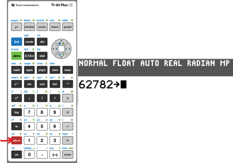






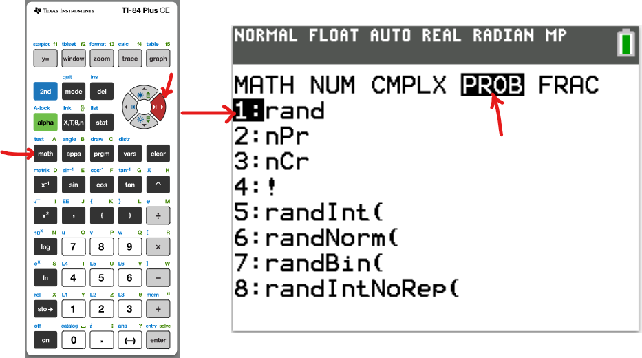
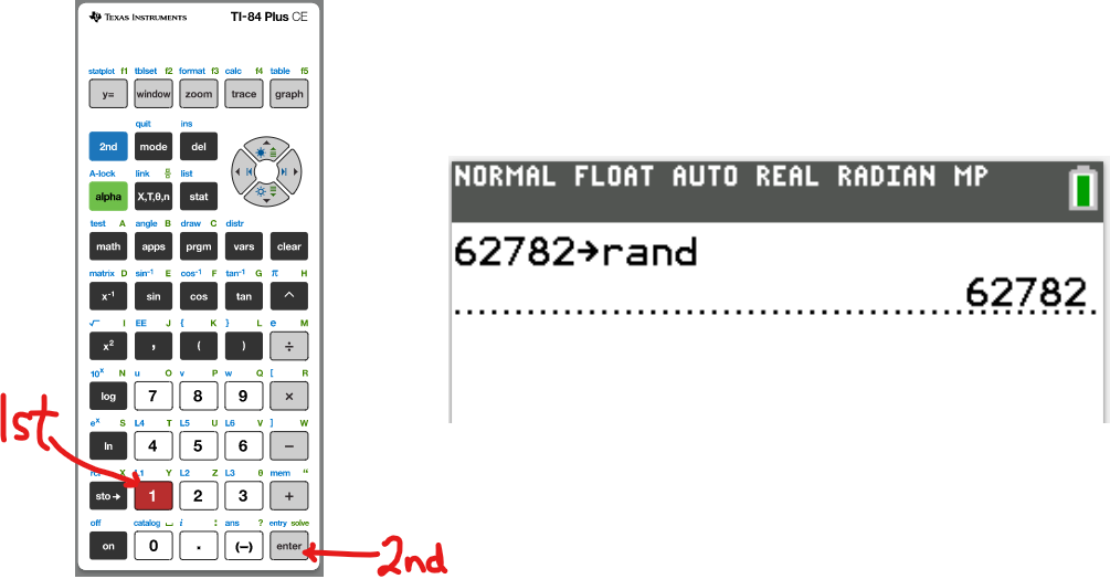
Because the songs are:
single digits
total of 9
selection of 3:
We shall use:
lower = 1
upper = 9
number, n = 3
(2.) Select 3 songs from 9 songs








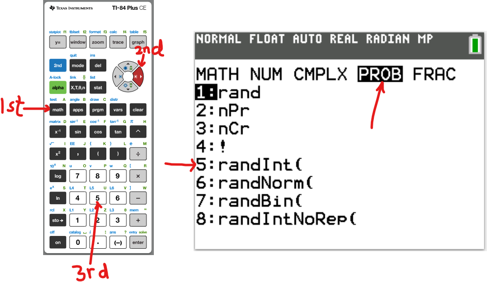
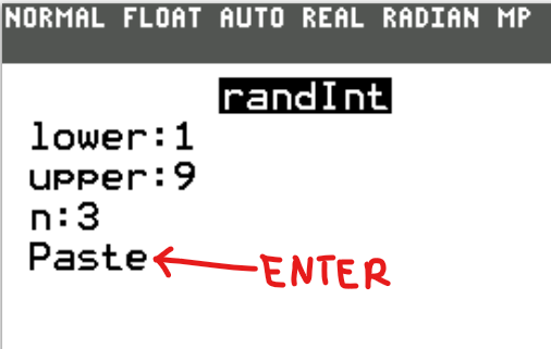
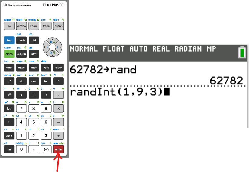
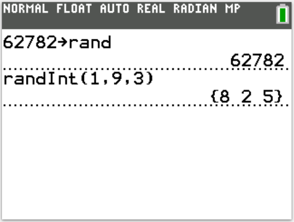
Student: What if a number repeats?
Teacher: We would use the No Repeat command: Number 8: randIntNoRep

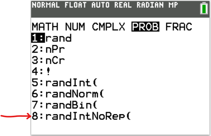
Generating Random Numbers Using Pearson StatCrunch

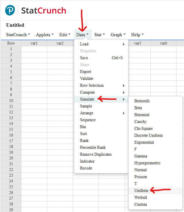
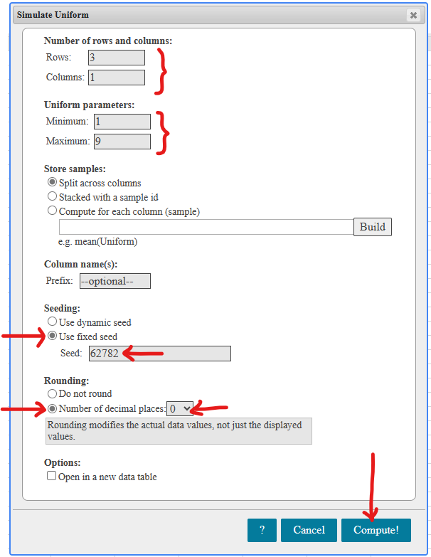
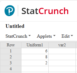
(15.) The manager of Samdom For Peace Apartments has a list of the names of 438 residents living in the east wing of the main apartment.
He intends to conduct an opinion survey of resident services.
Use the portion of the Table of Random Numbers below to produce five different three-digit numbers corresponding to the names selected.
Begin with the first column of the first row and work down each column.

Table of Random Numbers
$79651$	$75929$
$31992$	$37168$
$64880$	$01006$
$99251$	$59613$
$42118$	$05606$
$29102$	$21720$
$26945$	$49265$
$42999$	$51017$
$17845$	$13429$
$58116$	$29876$

Show/Hide Answer

(2.) Stratified Sampling: This is a sampling technique in which the stratified sample is obtained by:
separating the population into non-overlapping groups known as strata, and
obtaining a simple random sample from each stratum.
Teacher: Singular is Stratum; Plural is Strata

The individuals within each stratum should be homogenous.
This means that the individuals within each stratum should have similar characteristics such as gender, class, and race among others.

Examples are:
(a.) Mr. C wants to know the average number of days in which the mathematics students at AWC were absent during a semester. He visited each math class on a certain day when the class is in session, and randomly selects $7$ students from each class.

(b.) Reuters poll conducted an election opinion poll of $25,000$ prospective voters for the Presidential election. They sorted out female responses to observe the candidates rankings with women.

(c.) Several pieces of fruit from each tree in an orchard are selected.

(3.) Cluster Sampling: This is a sampling technique in which the cluster sample is obtained by:
dividing the population into sections known as clusters,
randomly selecting some of those clusters, and
selecting all the individuals from those selected clusters.
Cluster sampling is similar to stratified sampling in the sense that the population is divided into groups. However, in cluster sampling; the entire individuals in those clusters are selected.

Examples are:
(a.) Mr. C is teaching a large class. He wants to know whether his students do their WebAssign homework assignments. 😊 He randomly selects $3$ rows out of the 7 rows of students in his class and asked all the students in those rows to show him the solutions of a certain homework assignment.

(b.) In a bid to improve its customer service, the management of a retail store randomly selects $50$ stores during a certain week. All customers present at those stores during that week are interviewed.

(4.) Systematic Sampling: This is a sampling technique in which the systematic sample is obtained by selecting every $kth$ individual from the population.
Begin from a starting point, then select every kth individual.
That starting point or individual corresponds to a random number between 1 and k.
To obtain a systematic sample with high validity, there must be a sampling frame as a randomly ordered list.

Examples are:
(a.) BeGood Computers produces laptops. To estimate the percentage of defects in a certain batch, the quality control manager starts from the $3^{rd}$ laptop, and selects every 12th laptop from the assembly line.

(b.) The people greeter at a certain Walmart store asks every outgoing 7th customer his/her shopping experience.

(c.) A telemarketer calls every 52nd person in a phone book directory that has over $100,000$ phone number listings of the residents of a city.

(5.) Multistage Sampling: This is a sampling technique in which samples are selected by a combination of two or more different sampling techniques, or a combination of the same sampling technique at different stages.
It consists of several stages (hence the name, "multistage") where each stage could comprise a particular sampling technique. Most large-scale surveys obtain samples using a combination of sampling techniques.

Examples are:
(a.) Micah Research Company wants to obtain a sample of undergraduate students in the United States. They used a simple random sample to select 12 states. From each of the selected states, 12 colleges or universities were chosen at random. Then, from each of the $144$ colleges or universities; a simple random sample of $30$ undergraduate students were selected.

(b.) Nielsen Media Research is an American firm that measures media audiences. They randomly select households and use an electronic box, called the People Meter to monitor the programs viewed by the households. They sell the information they obtain to television stations and companies. These results are helpful in determining the prices for commercials. How do they select these households?
First Stage: Stratified Sampling: They divide the country into geographical areas or strata using the U.S Census data. The strata typically consists of city blocks in urban areas and geographic regions in rural areas.
Second Stage: Simple Random Sampling: They send representatives to the selected strata and lists the households within the strata. The households are then randomly selected using a simple random sample.

(c.) Another good example of multistage sampling is the one used by the U.S Census Bureau for the CPS (Current Population Survey) .

Note: A census includes the entire population while a sampling includes only part of the population.

(6.) Convenience Sampling: This is a sampling technique in which the individuals in the convenience sample (also known as a voluntary response sample) are easily obtained because the individuals volunteered, rather than by randomness.
Begin from a starting point, then select every $kth$ individual.
The individuals in the sample voluntarily decide to participate in the survey.

Examples are:
(a.) America's Got Talent asked its viewers to vote for the contestant with the best performance. Some voted. Some did not.

(b.) Micaiah resides in the community of Happyland, Oklahoma. As part of his Statistics project, he would like to collect data on household size in his city. He asks each person in his class for the size of their household and then reports a simple random sample.

Teacher: Due to the fact that the individuals in this sample were not selected by randomness, do you think this sample is a representative of the population?
Do you think the results obtained from this sample are free from bias?
Do you think the results should be valid?
Please note the students' responses.

Exercise 5
Identify the sampling methods in these scenarios.
Explain what is wrong with the sampling method as applicable.

(16.) All $30$ students in Mr. C's Statistics class were asked to complete a survey to evaluate his teaching/instruction.
Of those $30$ students, only $10\%$ responded.

Show/Hide Answer

Bias in Sampling

Exercise 6
Determine whether the source has the potential to create a bias in a statistical study.

(17.) Opposition to Breast-Feeding Resolution by U.S. Stuns World Health Officials - New York Times
A resolution to encourage breast-feeding was expected to be approved quickly and easily by the hundreds of government delegates who gathered in the Spring of 2018 in Geneva for the United Nations-affiliated World Health Assembly.
But, the United States delegation, embracing the interests of infant formula manufacturers, upended the deliberations.

Show/Hide Answer

(18.) Georgia Northwestern Technical College (GNTC) obtained word counts from the most popular novels of the past three years.

Show/Hide Answer

Exercise 7
Determine whether these questions are biased or not.
If they are biased, write a less biased question.

(19.) Should companies that pollute the environment be forced to pay the costs of cleanup?

Show/Hide Answer

Data Organization

---

Objectives

Students will:
(1.) Organize raw data in classes using a frequency distribution table.
(2.) Compute the statistical properties of data.
(3.) Compute the relative frequencies of data.
(4.) Construct a relative frequency distribution table.
(5.) Compute the cumulative frequencies of data.
(6.) Construct a cumulative frequency distribution table.

Vocabulary Words

frequency distribution table, frequency table, class, classes, frequency, data set, class width, tally, class size, range, number of classes, maximum value, minimum value, class interval, class limit, lower class interval, lower class limit, upper class interval, upper class limit, class midpoint, class mark, class boundary, relative frequency, proportion, cumulative frequency

A Frequency Distribution Table also known as a Frequency Table is used to organize data.
It organizes a data set by:
(1.) Separating the data value in classes and
(2.) Listing the frequencies of each class.
It helps us to understand the nature of the distribution of the a data set.

Example 1
A Good Samaritan (generous giver) asked for the pant/trouser sizes of the staff at Divine Mercy Orphanage.
The raw data of the sizes are listed as shown:

Pant/Trouser Sizes
$36$ $44$ $42$ $36$ $42$	$38$ $48$ $48$ $40$ $42$	$42$ $42$ $42$ $48$ $42$	$40$ $48$ $48$ $46$ $44$	$50$ $38$ $32$ $44$ $42$	$48$ $42$ $36$ $40$ $42$	$48$ $44$ $44$ $46$ $42$

$(a.)$ Draw a frequency distribution table for the data. Your table should have $7$ classes.
$(b.)$ Compute the statistical properties of the classes.

Solution

1st Step: We want 7 classes.
So, we need to find the class width that will give us 7 classes.

Class Width is also known as Class Size.
Class Size is the size of the class.
We shall write Five Formulas for the Class Width

First Formula for Class Width

$ Class\:\:Width = \dfrac{Range}{Number\:\:of\:\:classes} \\[5ex] Range = Maximum - Minimum \\[3ex] \therefore Class\:\:Width = \dfrac{Maximum - Minimum}{Number\:\:of\:\:classes} \\[5ex] Maximum\:\:data\:\:value = 50 \\[3ex] Minimum\:\:data\:\:value = 32 \\[3ex] Class\:\:Width = \dfrac{50 - 32}{7} = \dfrac{18}{7} = 2.57 \\[5ex] $ 2nd Step: We need to round up the class width to the nearest integer.
This is the common rule.

Each class has a range of values, which are called Class Intervals
Class Interval is also known as Class Limit.
Class Intervals separates the classes, but with gaps between the classes.

The smallest data value of each class is the Lower Class Interval($LCI$) of that class
The highest data value of each class is the Upper Class Interval($UCI$) of that class

Second Formula for Class Width

$ Class\:\:Width = LCI\:\:of\:\:2nd\:\:Class - LCI\:\:of\:\:1st\:\:Class \\[3ex] \rightarrow LCI\:\:of\:\:2nd\:\:Class = LCI\:\:of\:\:1st\:\:Class + Class\:\:Width \\[5ex] $ 3rd Step: Let us write the lower class interval of the first class by choosing the minimum data value or any convenient value below the minimum.
Then, we write the lower class intervals of the remaining classes.

Student: Choosing the minimum data value or any convenient value below the minimum value?
May you please elaborate?
Teacher: Yes. In our example, we shall use the minimum data value.
However, in some cases - depending on the number of classes; we will need to use a value below the minimum value.
Student: When do we have such a case? May you give an example?
Teacher: If you are given the number of classes but not given the class size, then you calculate the class size using the first formula we just used.
Then, you try to use the minimum value (just as we shall use) and the second formula to write the first class. We then write other classes until you get to the class that also contains the maximum value. That class will be our final class.
Then, count the classes. If the number of classes is what is needed, then you did it well.
If the number of classes is greater or smaller than the required number of classes, then you will need to adjust the lower class interval of the first class. Please ensure that the first class contains the minimum value, just as the last class contains the maximum value.
Let us solve some examples where we shall just use the minimum value as the lower class interval of our first class. Then, we shall solve examples where we need to adjust the value of the class size as the lower class interval of the first class.
Please review the Solved Examples for at least an example of such cases.

So, let us write the lower class intervals of the classes.

$ LCI\:\:of\:\:1st\:\:Class = Minimum\:\:value = 32 \\[3ex] $ From the Second Formula for Class Width

$ LCI\:\:of\:\:2nd\:\:Class = LCI\:\:of\:\:1st\:\:Class + Class\:\:Width \\[3ex] LCI\:\:of\:\:3rd\:\:Class = LCI\:\:of\:\:2nd\:\:Class + Class\:\:Width \\[3ex] Class\:\:Width = 3 \\[3ex] LCI\:\:of\:\:2nd\:\:Class = 32 + 3 = 35 \\[3ex] Similarly \\[3ex] LCI\:\:of\:\:3rd\:\:Class = 35 + 3 = 38 \\[3ex] LCI\:\:of\:\:4th\:\:Class = 38 + 3 = 41 \\[3ex] LCI\:\:of\:\:5th\:\:Class = 41 + 3 = 44 \\[3ex] LCI\:\:of\:\:6th\:\:Class = 44 + 3 = 47 \\[3ex] LCI\:\:of\:\:7th\:\:Class = 47 + 3 = 50 \\[5ex] $

4th Step: Let us write the upper class interval ($UCI$) of the first class by noting some rules.
Then, we write the upper class intervals of the remaining classes.
What are those rules?
Let us get back to Class Intervals
Recall that class intervals separate the classes, but with gaps between the classes.

NOTE:
(1.) If the class intervals (the $LCI$ and the $UCI$) are integers, then the difference between the lower class interval of a class and the upper class interval of the previous/preceding class is $1$

$ LCI\:\:of\:\:2nd\:\:Class - UCI\:\:of\:\:1st\:\:Class = 1 \\[3ex] LCI\:\:of\:\:5th\:\:Class - UCI\:\:of\:\:4th\:\:Class = 1 \\[3ex] LCI\:\:of\:\:8th\:\:Class - UCI\:\:of\:\:7th\:\:Class = 1 \\[5ex] $ (2.) If the class intervals (the $LCI$ and the $UCI$) are decimals rounded to one decimal place, then the difference between the lower class interval of a class and the upper class interval of the previous class is $0.1$

$ LCI\:\:of\:\:3rd\:\:Class - UCI\:\:of\:\:2nd\:\:Class = 0.1 \\[3ex] LCI\:\:of\:\:6th\:\:Class - UCI\:\:of\:\:5th\:\:Class = 0.1 \\[3ex] LCI\:\:of\:\:10th\:\:Class - UCI\:\:of\:\:9th\:\:Class = 0.1 \\[5ex] $ (3.) If the class intervals (the $LCI$ and the $UCI$) are decimals rounded to two decimal places, then the difference between the lower class interval of a class and the upper class interval of the previous class is $0.01$

$ LCI\:\:of\:\:4th\:\:Class - UCI\:\:of\:\:3rd\:\:Class = 0.01 \\[3ex] LCI\:\:of\:\:13th\:\:Class - UCI\:\:of\:\:12th\:\:Class = 0.01 \\[3ex] LCI\:\:of\:\:21st\:\:Class - UCI\:\:of\:\:20th\:\:Class = 0.01 \\[5ex] $ and so on and so forth.

In this case (our data values are integers):

$ LCI\:\:of\:\:2nd\:\:Class - UCI\:\:of\:\:1st\:\:Class = 1 \\[3ex] LCI\:\:of\:\:2nd\:\:Class = 35 \\[3ex] \rightarrow 35 - UCI\:\:of\:\:1st\:\:Class = 1 \\[3ex] UCI\:\:of\:\:1st\:\:Class = 35 - 1 \\[3ex] UCI = 34 \\[3ex] Recall\:\: LCI\:\:of\:\:1st\:\:Class = Minimum\:\:value = 32 \\[3ex] \therefore 1st\:\:Class = 32 - 34 \\[5ex] $ Third Formula for Class Width

$ Class\:\:Width = UCI\:\:of\:\:2nd\:\:Class - UCI\:\:of\:\:1st\:\:Class \\[3ex] \rightarrow UCI\:\:of\:\:2nd\:\:Class = UCI\:\:of\:\:1st\:\:Class + Class\:\:Width \\[3ex] UCI\:\:of\:\:3rd\:\:Class = UCI\:\:of\:\:2nd\:\:Class + Class\:\:Width \\[3ex] Class\:\:Width = 3 \\[3ex] UCI\:\:of\:\:2nd\:\:Class = 34 + 3 = 37 \\[3ex] Similarly \\[3ex] UCI\:\:of\:\:3rd\:\:Class = 37 + 3 = 40 \\[3ex] UCI\:\:of\:\:4th\:\:Class = 40 + 3 = 43 \\[3ex] UCI\:\:of\:\:5th\:\:Class = 43 + 3 = 46 \\[3ex] UCI\:\:of\:\:6th\:\:Class = 46 + 3 = 49 \\[3ex] UCI\:\:of\:\:7th\:\:Class = 49 + 3 = 52 \\[5ex] $

So, our classes are:

$ 1st\:\:Class:\:\: 32 - 34 \\[3ex] 2nd\:\:Class:\:\: 35 - 37 \\[3ex] 3rd\:\:Class:\:\: 38 - 40 \\[3ex] 4th\:\:Class:\:\: 41 - 43 \\[3ex] 5th\:\:Class:\:\: 44 - 46 \\[3ex] 6th\:\:Class:\:\: 47 - 49 \\[3ex] 7th\:\:Class:\:\: 50 - 52 \\[5ex] $

So, we have written the seven classes.
But, let us compute the statistical properties of these classes.
These include: class midpoints, class boundaries, relative frequencies, and cumulative frequencies for each class.

5th Step: Let us write the midpoints of each class.
Class Midpoints are also known as Class Marks
Class Midpoints are the midpoints of the classes.

Formula for Class Midpoint

$ Class\:\:Midpoint = \dfrac{LCI + UCI}{2} \\[5ex] 1st\:\:Class:\:\: Class\:\:Midpoint = \dfrac{32 + 34}{2} = \dfrac{66}{2} = 33 \\[5ex] 2nd\:\:Class:\:\: Class\:\:Midpoint = \dfrac{35 + 37}{2} = \dfrac{72}{2} = 36 \\[5ex] 3rd\:\:Class:\:\: Class\:\:Midpoint = \dfrac{38 + 40}{2} = \dfrac{78}{2} = 39 \\[5ex] 4th\:\:Class:\:\: Class\:\:Midpoint = \dfrac{41 + 43}{2} = \dfrac{84}{2} = 42 \\[5ex] 5th\:\:Class:\:\: Class\:\:Midpoint = \dfrac{44 + 46}{2} = \dfrac{90}{2} = 45 \\[5ex] 6th\:\:Class:\:\: Class\:\:Midpoint = \dfrac{47 + 49}{2} = \dfrac{96}{2} = 48 \\[5ex] 7th\:\:Class:\:\: Class\:\:Midpoint = \dfrac{50 + 52}{2} = \dfrac{102}{2} = 51 \\[5ex] $

Student: I just noticed a pattern with the class midpoints and the class width
Teacher: Good observation. However, please use the formula I gave you.
Do not use a shortcut of finding the class midpoint of the first class and adding the class width to find the class midpoints of the remaining classes.
It is not the formula/technique we use for finding the class midpoints, even though the technique worked in this case. It does not work all the time.

Recall: Class Intervals separate the classes, but with gaps between the classes.
What about any statistical property that does not have any gaps between the classes?
What statistical property takes into account "all" the data...especially for continuous data?
For example: In the first two classes:
First class: $32 - \color{red}{34}$
Second Class: $\color{red}{35} - 37$
What happens to the data values between $34$ and $35$?
This brings us to...

6th Step: Let us write the class boundary of each class.
Class Boundaries separate the classes, but without gaps between the classes.
The Class Boundary for each class comprise the Lower Class Boundary, $LCB$ and the Upper Class Boundary, $UCB$
Formula for Class Boundaries

$ Lower\:\:Class\:\:Boundary\:\:of\:\:a\:\:class = \dfrac{LCI\:\:of\:\:that\:\:class + UCI\:\:of\:\:previous/preceding\:\:class}{2} \\[5ex] Upper\:\:Class\:\:Boundary\:\:of\:\:a\:\:class = \dfrac{UCI\:\:of\:\:that\:\:class + LCI\:\:of\:\:next/succeeding\:\:class}{2} \\[5ex] LCB\:\:of\:\:2nd\:\:Class = \dfrac{LCI\:\:of\:\:2nd\:\:Class + UCI\:\:of\:\:1st\:\:Class}{2} = \dfrac{35 + 34}{2} = \dfrac{69}{2} = 34.5 \\[5ex] UCB\:\:of\:\:2nd\:\:Class = \dfrac{UCI\:\:of\:\:2nd\:\:Class + LCI\:\:of\:\:3rd\:\:Class}{2} = \dfrac{37 + 38}{2} = \dfrac{75}{2} = 37.5 \\[5ex] Class\:\:Boundary\:\:of\:\:2nd\:\:Class = 34.5 - 37.5 \\[3ex] LCB\:\:of\:\:3rd\:\:Class = \dfrac{LCI\:\:of\:\:3rd\:\:Class + UCI\:\:of\:\:2nd\:\:Class}{2} = \dfrac{38 + 37}{2} = \dfrac{69}{2} = 37.5 \\[5ex] UCB\:\:of\:\:3rd\:\:Class = \dfrac{UCI\:\:of\:\:3rd\:\:Class + LCI\:\:of\:\:4th\:\:Class}{2} = \dfrac{40 + 41}{2} = \dfrac{81}{2} = 40.5 \\[5ex] Class\:\:Boundary\:\:of\:\:3rd\:\:Class = 37.5 - 40.5 \\[5ex] $

Student: What about the class boundary of the first class?
Teacher: Good question.
What do you think?
Student: I think the $UCB$ of the first class would be: $34.5$
Teacher: That is correct.
How did you get it?
From the formula?
Student: No. I noticed that the $UCB$ of the first class should be the $LCB$ of the second class because there are no gaps between the classes. Is that right?
Teacher: That is very correct...and good reasoning.
But, you can also get it from the formula I gave you.
Student: Yes, I know.
But, how do we get the $LCB$ of the first class?

What about the class boundary of the first class?

$ UCB\:\:of\:\:1st\:\:Class = \dfrac{UCI\:\:of\:\:1st\:\:Class + LCI\:\:of\:\:2nd\:\:Class}{2} = \dfrac{34 + 35}{2} = \dfrac{69}{2} = 34.5 \\[5ex] $ But, how do we write the lower class boundary of the first class?

$ LCB\:\:of\:\:1st\:\:Class = \dfrac{LCI\:\:of\:\:1st\:\:Class + UCI\:\:of\:\:previous\:\:Class}{2} \\[5ex] $ We do not have a previous class.
But, assuming we did; the $UCI$ of that class would be $34 - 3 = 31$

$ \therefore LCB\:\:of\:\:1st\:\:Class = \dfrac{32 + 31}{2} = \dfrac{63}{2} = 31.5 \\[5ex] Class\:\:Boundary\:\:of\:\:1st\:\:Class = 31.5 - 34.5 \\[3ex] $ Also, how do we write the upper class boundary of the seventh class?

$ UCB\:\:of\:\:7th\:\:Class = \dfrac{UCI\:\:of\:\:7th\:\:Class + LCI\:\:of\:\:next\:\:Class}{2} \\[5ex] $ We do not have a next class.
But, assuming we did; the $LCI$ of that class would be $50 + 3 = 53$

$ \therefore UCB\:\:of\:\:7th\:\:Class = \dfrac{52 + 53}{2} = \dfrac{105}{2} = 52.5 \\[5ex] Class\:\:Boundary\:\:of\:\:7th\:\:Class = 49.5 - 52.5 \\[3ex] $

Teacher: Did you notice any relationship between the class boundary and the class width?
Student: Yes.
The class width is the difference between the upper class boundary and the lower class boundary of the same class.
Teacher: That is very correct.
This leads us to write the...

Fourth Formula for Class Width

$ Class\:\:Width = UCB\:\:of\:\:a\:\:class - LCB\:\:of\:\:the\:\:same\:\:class \\[3ex] UCB\:\:of\:\:a\:\:class - LCB\:\:of\:\:the\:\:same\:\:class = Class\:\:Width \\[3ex] \rightarrow UCB\:\:of\:\:a\:\:class = Class\:\:Width + LCB\:\:of\:\:the\:\:same\:\:class \\[3ex] UCB\:\:of\:\:a\:\:class = LCB\:\:of\:\:the\:\:same\:\:class + Class\:\:Width \\[3ex] Class\:\:Width = UCB\:\:of\:\:1st\:\:Class - LCB\:\:of\:\:1st\:\:Class = 34.5 - 31.5 = 3 \\[3ex] Class\:\:Width = UCB\:\:of\:\:2nd\:\:Class - LCB\:\:of\:\:2nd\:\:Class = 37.5 - 34.5 = 3 \\[3ex] $ Because class boundaries do not have gaps between the classes, we notice that:

$ UCB\:\:of\:\:1st\:\:Class = LCB\:\:of\:\:2nd\:\:Class \\[3ex] UCB\:\:of\:\:2nd\:\:Class = LCB\:\:of\:\:3rd\:\:Class \\[3ex] This\:\:implies\:\:that \\[3ex] LCB\:\:of\:\:1st\:\:Class = LCB\:\:of\:\:2nd\:\:Class - Class\:\:Width \\[3ex] Also \\[3ex] UCB\:\:of\:\:7th\:\:Class = UCB\:\:of\:\:6th\:\:Class + Class\:\:Width \\[3ex] $ This leads us to another formula for class width.

Fifth Formula for Class Width

$ Class\:\:Width = LCB\:\:of\:\:a\:\:Class - LCB\:\:of\:\:previous\:\:class \\[3ex] \rightarrow LCB\:\:of\:\:a\:\:Class = LCB\:\:of\:\:previous\:\:class + Class\:\:Width \\[3ex] Class\:\:Width = UCB\:\:of\:\:a\:\:Class - UCB\:\:of\:\:previous\:\:class \\[3ex] \rightarrow UCB\:\:of\:\:a\:\:Class = UCB\:\:of\:\:previous\:\:class + Class\:\:Width \\[3ex] $ Let us write the lower class boundaries of the remaining classes.

$ LCB\:\:of\:\:3rd\:\:Class = LCB\:\:of\:\:2nd\:\:Class + Class\:\:Width \\[3ex] LCB\:\:of\:\:3rd\:\:Class = 34.5 + 3 = 37.5 \\[3ex] Similarly \\[3ex] LCB\:\:of\:\:4th\:\:Class = 37.5 + 3 = 40.5 \\[3ex] LCB\:\:of\:\:5th\:\:Class = 40.5 + 3 = 43.5 \\[3ex] LCB\:\:of\:\:6th\:\:Class = 43.5 + 3 = 46.5 \\[3ex] LCB\:\:of\:\:7th\:\:Class = 46.5 + 3 = 49.5 \\[3ex] $ Let us write the upper class boundaries of the remaining classes.

$ UCB\:\:of\:\:3rd\:\:Class = UCB\:\:of\:\:2nd\:\:Class + Class\:\:Width \\[3ex] UCB\:\:of\:\:3rd\:\:Class = 37.5 + 3 = 40.5 \\[3ex] Similarly \\[3ex] UCB\:\:of\:\:4th\:\:Class = 40.5 + 3 = 43.5 \\[3ex] UCB\:\:of\:\:5th\:\:Class = 43.5 + 3 = 46.5 \\[3ex] UCB\:\:of\:\:6th\:\:Class = 46.5 + 3 = 49.5 \\[3ex] UCB\:\:of\:\:7th\:\:Class = 49.5 + 3 = 52.5 \\[5ex] $

$\boldsymbol{7th\:\:Step}$ Let us write the relative frequency of each class.
Relative Frequency, $RF$ (also known as Proportion) of a class is the ratio of the frequency of that class to the total frequency of the data set.
It is the proportion of the observations that display the relevant characteristic.
It is used in summarizing a distribution.
Formula for Relative Frequency

$ RF\:\:of\:\:a\:\:class = \dfrac{Frequency\:\:of\:\:that\:\:class}{\Sigma F} \\[5ex] \Sigma F \:\:means\:\:summation\:\:of\:\:the\:\:frequencies \\[3ex] RF\:\:of\:\:3rd\:\:Class = \dfrac{Frequency\:\:of\:\:3rd\:\:Class}{\Sigma F} \\[5ex] $ Relative Frequency of a class is expressed as a fraction, decimal, or percent.
The sum of the relative frequencies of all the classes should be equal to $100\%$ or $1$

$ \Sigma RF = 100\% \\[3ex] \Sigma RF = 1 \\[3ex] $ We shall calculate the relative frequencies in the Frequency Table.

$\boldsymbol{8th\:\:Step}$ Let us write the cumulative frequency of each class.
Cumulative Frequency, $CF$ of a class is the sum of the frequencies prior to that class and the frequency of that class.
Formula for Cumulative Frequency

$ CF\:\:of\:\:1st\:\:Class = Frequency\:\:of\:\:1st\:\:Class \\[3ex] CF\:\:of\:\:2nd\:\:Class = Frequency\:\:of\:\:1st\:\:Class + Frequency\:\:of\:\:2nd\:\:Class \\[3ex] CF\:\:of\:\:3rd\:\:Class = Frequency\:\:of\:\:1st\:\:Class + Frequency\:\:of\:\:2nd\:\:Class + Frequency\:\:of\:\:3rd\:\:Class \\[3ex] $ The last cumulative frequency (the cumulative frequency of the last class) is the sum of all the frequencies.

$Last\:\:CF = CF\:\:of\:\:Last\:\:Class = \Sigma F \\[3ex]$ We shall calculate the cumulative frequencies in the Frequency Table.

The Frequency Distribution Table is drawn as shown:

Class Intervals	Tally	Frequency, $F$	Class Midpoints	Class Boundaries	Relative Frequency, $RF$	Cumulative Frequency, $CF$
$32 - 34$	I	$1$	$33$	$31.5 - 34.5$	$\dfrac{1}{35} = 0.02875 = 2.875\%$	$1$
$35 - 37$	III	$3$	$36$	$34.5 - 37.5$	$\dfrac{3}{35} = 0.08571 = 8.571\%$	$1 + 3 = 4$
$38 - 40$	IIII	$5$	$39$	$37.5 - 40.5$	$\dfrac{5}{35} = \dfrac{1}{7} = 0.14286 = 14.286\%$	$4 + 5 = 9$
$41 - 43$	IIII IIII I	$11$	$42$	$40.5 - 43.5$	$\dfrac{11}{35} = 0.31429 = 31.429\%$	$9 + 11 = 20$
$44 - 46$	IIII II	$7$	$45$	$43.5 - 46.5$	$\dfrac{7}{35} = \dfrac{1}{5} = 0.2 = 20\%$	$20 + 7 = 27$
$47 - 49$	IIII II	$7$	$48$	$46.5 - 49.5$	$\dfrac{7}{35} = \dfrac{1}{5} = 0.2 = 20\%$	$27 + 7 = 34$
$50 - 52$	I	$1$	$51$	$49.5 - 52.5$	$\dfrac{1}{35} = 0.02875 = 2.875\%$	$34 + 1 = \color{red}{35}$
		$\Sigma F = \color{red}{35}$			$\Sigma RF = 1 = 100\%$

CHECKS
$(1.)$ The summation of the frequencies, $\Sigma F$ is equal to the sample size.
$(2.)$ The summation of relative frequencies, $\Sigma RF$ is equal to $1$ or $100\%$
$(3.)$ The value in the last row of the cumulative frequency should be the same value as the summation of the frequencies (as noted by the red color in the table)

MORE NOTES
$(1.)$ If the number of classes is given but the class width is not given, use a class width that would give an ideal (a reasonable) number of classes.

$(2.)$ If the class width is given, use the class width.

$(3.)$ If the number of classes and the class width are given but the class width did not give that number of classes; then adjust the class width to give the required number of classes.
Unless otherwise specified by your professor, do not create classes as you wish. Adjust the class size to give the required number of classes.

$(4.)$ The first class must contain the smallest data value (minimum value).

$(5.)$ The last class must contain the highest data value (maximum value).

$(6.)$ Each class must be uniform. In other words, the class width/class size must be the same.

$(7.)$ Follow the directions specified by your professor on what should be in the frequency table. He/She grades your work.

Data Presentation

---

Objectives

Students will:
(1.) Represent data using several data presentation tools.
(2.) Calculate the sectorial angles of the variables in pie charts.
(3.) Calculate the percentages of the variables in pie charts.
(4.) Interpret the data presented with several data presentation tools.
(5.) Identify misleading graphs.
(6.) Correct misleading graphs.

Vocabulary Words

frequency distribution table, frequency table, dotplot, boxplot (also known as box-and-whisker plot), stemplot (stem-and-leaf plot), scatter plot, scatter diagram, normal quantile plot, quantile-quantile plot, QQ plot, line graph, bar graph, bar chart, circle graph, pie chart, cumulative frequency graph, ogive, cumulative frequency curve, Pareto chart, pictogram, histogram, frequency polygon, cumulative frequency polygon, percentages, two-way table, contour map

First identify whether the variable under investigation is numerical or categorical.
If the variable is​ numerical, a​ dotplot, histogram, or stemplot can be used.
If the variable is​ categorical, a bar​ chart, Pareto​ chart, or pie chart can be used. However, bar charts and pie charts are commonly used.
When describing the distribution of a categorical variable, the category that appears most often is the mode.
When summarizing graphs of categorical data, report the mode(s), and describe the variability.
If the distribution of a categorical variable has a lot of diversity or many observations in many different categories, the variability is high.
If the distribution has a little diversity, or if many observations fall into the same category, the variability is low.
Pay attention to the differences in the charts and which would be the best to display the specific data set.

The distribution of a sample organizes data by recording all the values observed in a sample and the number of times each value was observed.
The two-step process used to examine distributions are: See the data and Summarize it.
When examining a distribution, first: visualize or see the distribution; second: use characteristics of the visualization to summarize the data.
All methods used for visualizing distributions are based on making a mark that indicates the number of times each value occurs in the data set.


When examining a distribution of numerical data:
(1.) The shape, center, and spread need to be considered.

(2.) The three basic characteristics of the shape of the distribution are:
(a.) Symmetric or skewness of the distribution
(b.) The number of mounds that appear in the distribution (based on the number of modes of the dataset).
(c.) Presence of outliers (whether unusually large or small values are present). Outliers are extreme values that are so large or so small that they do not fit into the pattern of the distribution.

A right-skewed distribution is the distribution of a variable in which most of the values are relatively small but also has a few very large values.
The graphical representation of the distribution appear to have a tail that extends to the right.
For example: (1.) the number of hours of TV viewed by a sample of people in a week: the smallest possible value in this case is 0. Most values will likely cluster around a common value. However, the presence of a small number of people who view TV for long hours will make the distribution to be right-skewed.



Percentages or rates are often better than counts for making comparisons because they account for possible differences among the sizes of groups.
A two-way table is used to summarize two potentially related categorical variables.

A contour map can hone in on the trend the same way a regression line can.
It helps one see trends in the concentration on a map.

Histogram

Histograms produce a smooth graphic by grouping observations into intervals known as bins.
In a histogram, observations are grouped into intervals called bins.
Changing the width of bins in a histogram changes the shape of the histogram. Narrow bins results in a spiky histogram that shows a lot of detail, while wider bins hide more detail.

Bar Chart

For a bar chart:
The horizontal axis of the bar chart represents the categories of the​ distribution.

Bar Chart versus Histogram

	Bar Chart	Histogram
(1.)	It is best suited for presenting qualitative (categorical) variables.	It is best suited for presenting quantitative (numerical) variables.
(2.)	There are gaps between the bars.	Typically, there are no gaps between the bars unless no value was observed for that variable. If there is a gap, the gap indicates that no values were observed in the interval represented by the gap.
(3.)	It does not matter how wide or narrow the bars are.	The widths of the bars have meaning.
(4.)	Sometimes, it does not matter in which order the bars are placed.	The order of the placement of the bars matter. A histogram has bars in ascending order.

Stem-and-Leaf Plot (Stemplot)

A stem-and-leaf plot (also known as a stemplot) is preferably used for visualizing numerical variables when:
(1.) Technology is not available.
(2.) The data set is not large.
(3.) The actual values of the data need to be seen.

Pareto Chart

A Pareto chart is a bar chart that is sorted from most frequent to least frequent.

Pie Chart

Pie charts are not commonly used by statisticians or in scientific settings because the human eye has a difficult time judging how much area is taken up by it's wedge-shaped slice.

$ Sectorial\;\;\angle\;\;for\;\;each\;\;age\;\;group = \dfrac{frequency\;\;of\;\;the\;\;age\;\;group}{\Sigma f} * 100 \\[5ex] $

References

---

Chukwuemeka, Samuel Dominic (2023). Introductory Statistics Retrieved from https://mathematicscourses.github.io/Statistics/

Bennett, J. O., & Briggs, W. L. (2019). Using and Understanding Mathematics: A Quantitative Reasoning Approach. Pearson.

Black, Ken. (2012). Business Statistics for Contemporary Decision Making (7th ed.). New Jersey: Wiley

Gould, R., Wong, R., & Ryan, C. N. (2020). Introductory Statistics: Exploring the world through data (3rd ed.). Pearson.

Kozak, Kathryn. (2015). Statistics Using Technology (2nd ed.).

Larson, R. (2026). Elementary Statistics. Pearson.

OpenStax, Introductory Statistics.OpenStax CNX. Sep 28, 2016. Retrieved from https://cnx.org/contents/30189442-6998-4686-ac05-ed152b91b9de@18.12

Sullivan, M., & Barnett, R. (2013). Statistics: Informed decisions using data with an introduction to mathematics of finance (2nd custom ed.). Boston: Pearson Learning Solutions.

Triola, M. F. (2015). Elementary Statistics using the TI-83/84 Plus Calculator (5th ed.). Boston: Pearson

Triola, M. F. (2022). Elementary Statistics. (14th ed.) Hoboken: Pearson.

Weiss, Neil A. (2015). Elementary Statistics (9th ed.). Boston: Pearson

Authority (NZQA), (n.d.). Mathematics and Statistics subject resources. www.nzqa.govt.nz. Retrieved December 14, 2020, from https://www.nzqa.govt.nz/ncea/subjects/mathematics/levels/

CrackACT. (n.d.). Retrieved from http://www.crackact.com/act-downloads/

CMAT Question Papers CMAT Previous Year Question Bank - Careerindia. (n.d.). https://www.careerindia.com. Retrieved May 30, 2020, from https://www.careerindia.com/entrance-exam/cmat-question-papers-e23.html

CSEC Math Tutor. (n.d). Retrieved from https://www.csecmathtutor.com/past-papers.html

Desmos. (n.d.). Desmos Graphing Calculator. https://www.desmos.com/calculator

DLAP Website. (n.d.). Curriculum.gov.mt. https://curriculum.gov.mt/en/Examination-Papers/Pages/list_secondary_papers.aspx

Free Jamb Past Questions And Answer For All Subject 2020. (2020, January 31). Vastlearners. https://www.vastlearners.com/free-jamb-past-questions/

Geogebra. (2019). Graphing Calculator - GeoGebra. Geogebra.org. https://www.geogebra.org/graphing?lang=en

GCSE Exam Past Papers: Revision World. Retrieved April 6, 2020, from https://revisionworld.com/gcse-revision/gcse-exam-past-papers

HSC exam papers | NSW Education Standards. (2019). Nsw.edu.au. https://educationstandards.nsw.edu.au/wps/portal/nesa/11-12/resources/hsc-exam-papers

JAMB Past Questions, WAEC, NECO, Post UTME Past Questions. (n.d.). Nigerian Scholars. Retrieved February 12, 2022, from https://nigerianscholars.com/past-questions/

KCSE Past Papers by Subject with Answers-Marking Schemes. (n.d.). ATIKA SCHOOL. Retrieved June 16, 2022, from https://www.atikaschool.org/kcsepastpapersbysubject

Myschool e-Learning Centre - It's Time to Study! - Myschool. (n.d.). https://myschool.ng/classroom

Netrimedia. (2022, May 2). ICSE 10th Board Exam Previous Papers- Last 10 Years. Education Observer. https://www.educationobserver.com/icse-class10-previous-papers/

NSC Examinations. (n.d.). www.education.gov.za. https://www.education.gov.za/Curriculum/NationalSeniorCertificate(NSC)Examinations.aspx

Papua New Guinea: Department of Education. (n.d.). www.education.gov.pg. Retrieved November 24, 2020, from http://www.education.gov.pg/TISER/exams.html

School Curriculum and Standards Authority (SCSA): K-12. Past ATAR Course Examinations. Retrieved December 10, 2021, from https://senior-secondary.scsa.wa.edu.au/further-resources/past-atar-course-exams

TI Products | Calculators and Technology | Texas Instruments. (n.d.). Education.ti.com. Retrieved March 18, 2023, from https://education.ti.com/en/products

West African Examinations Council (WAEC). Retrieved May 30, 2020, from https://waeconline.org.ng/e-learning/Mathematics/mathsmain.html

51 Real SAT PDFs and List of 89 Real ACTs (Free) : McElroy Tutoring. (n.d.). Mcelroytutoring.com. Retrieved December 12, 2022, from https://mcelroytutoring.com/lower.php?url=44-official-sat-pdfs-and-82-official-act-pdf-practice-tests-free